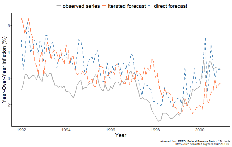
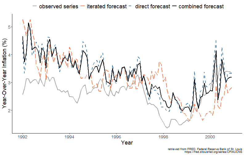
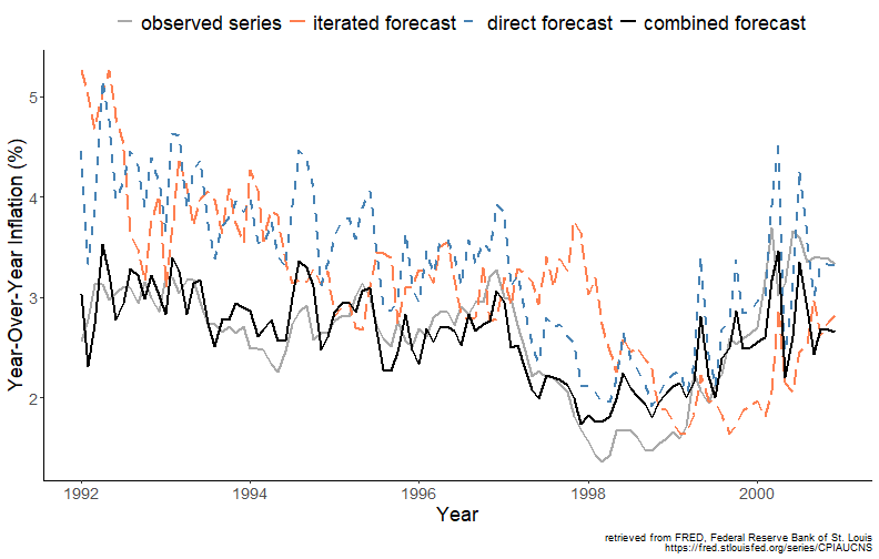
class: center, middle, inverse, title-slide .title[ # Forecasting for Economics and Business ] .subtitle[ ## Lecture 10: Forecast Combination ] .author[ ### David Ubilava ] .date[ ### University of Sydney ] --- # All forecasts are wrong, but a few may be useful .pull-left[  ] .pull-right[By choosing the most appropriate model for obtaining forecasts, we implicitly discard all other candidate models. Those models could potentially contain useful information that the chosen model cannot offer. Thus, merely selecting the best model may be a sub-optimal strategy. An alternative strategy is to use some information from all forecasts, i.e., *forecast combination*. ] --- # Why combine? .right-column[ Several factors support the idea of forecast combination: - The concept is intuitively appealing (a combined forecast aggregates more information or more ways of processing the information); - Many forecast combination techniques are computationally simple and easy to apply; - Empirical evidence strongly supports the idea of combining forecast to improve accuracy; - The concept of forecast combination leads naturally to the concept of *forecast encompassing* - a valuable tool in forecast evaluation. ] --- # How it works? .right-column[ Consider two forecasting methods (or models), `\(i\)` and `\(j\)`, each respectively yielding one-step-ahead forecasts `\(y_{t+1|t,i}\)` and `\(y_{t+1|t,j}\)`, and the associated forecast errors `\(e_{t+1,i} = y_{t+1}-y_{t+1|t,i}\)` and `\(e_{t+1,j} = y_{t+1}-y_{t+1|t,j}\)`. A combined forecast, `\(y_{t+1|t,c}\)`, is expressed as: `$$y_{t+1|t,c} = (1-\omega)y_{t+1|t,i} + \omega y_{t+1|t,j},$$` where `\(0 \leq \omega \leq 1\)` is a weight, and, thus, the combined forecast is a weighted average of the two individual forecasts. ] --- # A combined forecast error mean .right-column[ A combined forecast error is: `$$e_{t+1,c} = (1-\omega)e_{t+1,i} + \omega e_{t+1,j}$$` The mean of a combined forecast error (under the assumption of forecast error unbiasedness) is zero: `$$E\left(e_{t+1,c}\right) = E\left[(1-\omega)e_{t+1,i} + \omega e_{t+1,j}\right] = 0$$` ] --- # A combined forecast error variance .right-column[ The variance of a combined forecast error is: `$$Var\left(e_{t+1,c}\right) = (1-\omega)^2 \sigma_i^2 + \omega^2 \sigma_j^2 + 2\omega(1-\omega)\rho\sigma_i\sigma_j,$$` where `\(\sigma_i\)` and `\(\sigma_j\)` are the standard deviations of the forecast errors from models `\(i\)` and `\(j\)`, and `\(\rho\)` is a correlation between these two forecast errors. ] --- # The optimal weight .right-column[ Taking the derivative of the variance of a combined forecast error, and equating it to zero yields an optimal weight (which minimizes the combined forecast error variance): `$$\omega^* = \frac{\sigma_i^2-\rho\sigma_i\sigma_j}{\sigma_i^2+\sigma_j^2-2\rho\sigma_i\sigma_j}$$` ] --- # At least as efficient as individual forecasts .right-column[ Substitute `\(\omega^*\)` in place of `\(\omega\)` in the formula for variance to obtain: `$$Var\left[e_{t+1,c}(\omega^*)\right] = \sigma_c^2(\omega^*) = \frac{\sigma_i^2\sigma_j^2(1-\rho^2)}{\sigma_i^2+\sigma_j^2-2\rho\sigma_i\sigma_j}$$` It can be shown that `\(\sigma_c^2(\omega^*) \leq \min\{\sigma_i^2,\sigma_j^2\}\)`. That is to say that by combining forecasts we are not making things worse (so long as we use *optimal* weights). ] --- # Combination Weights—Special Cases ## Case 1: `\(\sigma_i = \sigma_j = \sigma\)`. .right-column[ Suppose the individual forecasts are equally accurate, then the combined forecast error variance reduces to: `$$\sigma_c^2(\omega^*) = \frac{\sigma^2(1+\rho)}{2} \leq \sigma^2$$` The equation shows there are diversification gains even when the forecasts are equally accurate (unless the forecasts are perfectly correlated, in which case there are no gains from combination). ] --- # Combination Weights—Special Cases ## Case 2: `\(\rho=0\)`. .right-column[ Suppose the forecast errors are uncorrelated, then the sample estimator of `\(\omega^*\)` is given by: `$$\omega^* = \frac{\sigma_i^2}{\sigma_i^2+\sigma_j^2} = \frac{\sigma_j^{-2}}{\sigma_i^{-2}+\sigma_j^{-2}}$$` Thus, the weights attached to forecasts are inversely proportional to the variance of these forecasts. ] --- # Combination Weights—Special Cases ## Case 3: `\(\sigma_i = \sigma_j = \sigma\)` and `\(\rho=0\)`. .right-column[ Suppose the individual forecasts are equally accurate and the forecast errors are uncorrelated, then the sample estimator of `\(\omega^*\)` reduces to `\(0.5\)`, resulting in the equal-weighted forecast combination: `$$y_{t+1|t,c} = 0.5y_{t+1|t,i} + 0.5y_{t+1|t,j}$$` ] --- # The sample optimal weight .right-column[ In practice `\(\sigma_i\)`, `\(\sigma_j\)`, and `\(\rho\)` are unknown. The sample estimator of `\(\omega^*\)` is: `$$\hat{\omega}^* = \frac{\hat{\sigma}_i^2-\hat{\sigma}_{ij}}{\hat{\sigma}_i^2+\hat{\sigma}_j^2-2\hat{\sigma}_{ij}},$$` where `\(\hat{\sigma}_i^2 = \frac{1}{P-1}\sum_{t=R}^{R+P-1}{e_{t+1,i}^2}\)` and `\(\hat{\sigma}_j^2 = \frac{1}{P-1}\sum_{t=R}^{R+P-1}{e_{t+1,j}^2}\)` are sample forecast error variances, and `\(\hat{\sigma}_{ij}=\frac{1}{P-1}\sum_{t=R}^{R+P-1}{e_{t+1,i}e_{t+1,j}}\)` is a sample forecast error covariance, where `\(P\)` denotes the number of out-of-sample forecasts. ] --- # The optimal weight in a regression setting .right-column[ The optimal weight has a straightforward interpretation in a regression setting. Consider the combined forecast equation as: `$$y_{t+1} = (1-\omega)y_{t+1|t,i} + \omega y_{t+1|t,j} + \varepsilon_{t+1},$$` where `\(\varepsilon_{t+1}\equiv e_{t+1,c}\)`. We can re-arrange the equation so that: `$$e_{t+1,i} = \omega (y_{t+1|t,j}-y_{t+1|t,i}) + \varepsilon_{t+1},$$` where `\(\omega\)` is obtained by estimating a linear regression with an intercept restricted to zero. ] --- # Direct and Iterated Forecasts of the U.S. Inflation .right-column[ <!-- --> ] --- # Regression-based optimal weights .right-column[ ``` ## ## t test of coefficients: ## ## Estimate Std. Error t value Pr(>|t|) ## I(dir - itr) 0.75417 0.19002 3.9689 0.0001303 *** ## --- ## Signif. codes: 0 '***' 0.001 '**' 0.01 '*' 0.05 '.' 0.1 ' ' 1 ``` ] --- # Regression-based optimal weights .right-column[ <!-- --> ] --- # The optimal weight in a regression setting .right-column[ Alternatively, we can estimate a variant of the combined forecast equation: `$$y_{t+1} = \alpha+\beta_i y_{t+1|t,i} + \beta_j y_{t+1|t,j} + \varepsilon_{t+1},$$` which relaxes the assumption of forecast unbiasedness, as well as of weights adding up to one or, indeed, of non-negative weights. ] --- # Regression-based optimal weights .right-column[ ``` ## ## t test of coefficients: ## ## Estimate Std. Error t value Pr(>|t|) ## (Intercept) 0.908025 0.309973 2.9294 0.004159 ** ## itr -0.159430 0.072151 -2.2097 0.029279 * ## dir 0.663267 0.087312 7.5965 1.268e-11 *** ## --- ## Signif. codes: 0 '***' 0.001 '**' 0.01 '*' 0.05 '.' 0.1 ' ' 1 ``` ] --- # Regression-based optimal weights .right-column[ <!-- --> ] --- # Forecast encompassing .right-column[ A special case of forecast combination is when `\(\omega=0\)`. Such an outcome (of the optimal weights) is known as forecast encompassing. It is said that `\(y_{t+1|t,i}\)` encompasses `\(y_{t+1|t,j}\)`, when given that the former is available, the latter provides no additional useful information. ] --- # Forecast encompassing .right-column[ This is equivalent of testing the null hypothesis of `\(\omega=0\)` in the combined forecast error equation, which, after rearranging terms, yields the following regression: `$$e_{t+1,i} = \omega\left(e_{t+1,i}-e_{t+1,j}\right)+\varepsilon_{t+1},\;~~t=R,\ldots,R+P-1$$` where `\(\varepsilon_{t+1}\equiv e_{t+1,c}\)`, and where `\(R\)` is the size of the (first) estimation window, and `\(P\)` is the number of out-of-sample forecasts generated. ] --- # Forecast encompassing in a regression setting .right-column[ We can test for the forecast encompassing by regressing the realized value on individual forecasts: `$$y_{t+1} = \alpha + \beta_1 y_{t+1|t,i} + \beta_2 y_{t+1|t,j} + \varepsilon_{t+1},$$` and testing the null hypothesis that `\(\beta_2=0\)`, given that `\(\beta_1=1\)`. ] --- # Readings .pull-left[  ] .pull-right[ Gonzalez-Rivera, Chapter 9 ]