Chapter 5 – Comparing Forecasts

5.1 The Need for the Forecast Evaluation
Among several available models we can select one that offers the superior in-sample fit (e.g., based on the AIC or SIC), and then apply this model to generate the forecasts.
A more sensible approach, at least from the standpoint of a forecaster, would be to assess goodness of fit in an out-of-sample setting. Recall that the model that offer the best in-sample fit doesn’t necessarily produce the most accurate out-of-sample forecasts, among the considered models. That is, for example, while a better in-sample fit can be achieved by incorporating additional parameters in the model, such more complex models extrapolate the estimated parameter uncertainty into the forecasts, thus sabotaging their accuracy.
Thus far we have applied the following algorithm to identify ‘the best’ among the competing forecasts:
- decide on a loss function (e.g., quadratic loss);
- obtain forecasts, the forecast errors, and the corresponding sample expected loss (e.g., root mean squared forecast error) for each model;
- rank the models on their sample expected loss values;
- select the model with the lowest sample expected loss.
But the loss function is a function of the random variable, and in practice we deal with sample information, so sampling variation needs to be taken into the account. Statistical methods of evaluation are, therefore, desirable (to say it mildly).
5.2 Relative Forecast Accuracy Tests
Here we will cover two tests for the hypothesis that two forecasts are equivalent, in the sense that the associated loss differential is not statistically significantly different from zero.
Consider a time series of length \(T\). Suppose \(h\)-step-ahead forecasts for periods \(R+h\) through \(T\) have been generated from two competing models \(i\) and \(j\): \(y_{t+h|t,i}\) and \(y_{t+h|t,j}\), with corresponding forecast errors: \(e_{t+h,i}\) and \(e_{t+h,j}\). The null hypothesis of equal predictive ability can be given in terms of the unconditional expectation of the loss differential: \[H_0: E\left[d(e_{t+h,ij})\right] = 0,\] where \(d(e_{t+h,ij}) = L(e_{t+h,i})-L(e_{t+h,j})\).
5.2.1 The Morgan-Granger-Newbold Test
The Morgan-Granger-Newbold (MGN) test is based on auxiliary variables: \(u_{1,t+h} = e_{t+h,i}-e_{t+h,j}\) and \(u_{2,t+h} = e_{t+h,i}+e_{t+h,j}\). It follows that: \[E(u_{1,t+h},u_{2,t+h}) = MSFE(i,t+h)-MSFE(j,t+h).\] Thus, the hypothesis of interest is equivalent to testing whether the two auxiliary variables are correlated.
The MGN test statistic is: \[\frac{r}{\sqrt{(P-1)^{-1}(1-r^2)}}\sim t_{P-1},\] where \(t_{P-1}\) is a Student t distribution with \(P-1\) degrees of freedom, \(P\) is the number of out-of-sample forecasts, and \[r=\frac{\sum_{t=R}^{T-h}{u_{1,t+h}u_{2,t+h}}}{\sqrt{\sum_{t=R}^{T-h}{u_{1,t+h}^2}\sum_{t=R}^{T-h}{u_{2,t+h}^2}}}\]
The MGN test relies on the assumption that forecast errors (of the forecasts to be compared) are unbiased, normally distributed, and uncorrelated (with each other). These are rather strict assumptions that are, often, violated in empirical applications.
5.2.2 The Diebold-Mariano Test
The Diebold-Mariano (DM) test, put forward by Diebold and Mariano (1995), relaxes the aforementioned requirements on the forecast errors. The DM test statistic is: \[\frac{\bar{d}_h}{\sqrt{\sigma_d^2/P}} \sim N(0,1),\] where \(\bar{d}_h=P^{-1}\sum_{t=R}^{T-h} d(e_{t+h,ij})\), and where \(P=T-R-h+1\) is the total number of forecasts generated using a rolling or recursive window scheme, for example.
A modified version of the DM statistic, due to Harvey, Leybourne, and Newbold (1997), addresses the finite sample properties of the test, so that: \[\sqrt{\frac{P+1-2h+P^{-1}h(h-1)}{P}}DM\sim t_{P-1},\] where \(t_{P-1}\) is a Student t distribution with \(P-1\) degrees of freedom.
In practice, the test of equal predictive ability can be applied within the framework of a regression model as follows: \[d_{t+h} = \delta + \upsilon_{t+h}\;~~t = R,\ldots,T-h,\] where \(d_{t+h} \equiv d(e_{t+h,ij})\). The null of equal predictive ability is equivalent of testing \(H_0: \delta = 0\) in the OLS setting. Moreover, because \(d_{t+h}\) may be serially correlated, autocorrelation consistent standard errors should be used for inference.
5.3 Forecasting Year-on-Year Monthly Inflation 12-steps-ahead
Two methods for generating multi-step-ahead forecasts from autoregressions, for example, are the iterated and direct methods. Each has advantages and disadvantages, and when the model is mis-specified, which more often than not tends to be the case, either of the two methods can yield more accurate forecasts. We will examine this using the U.S. year-on-year monthly inflation data.
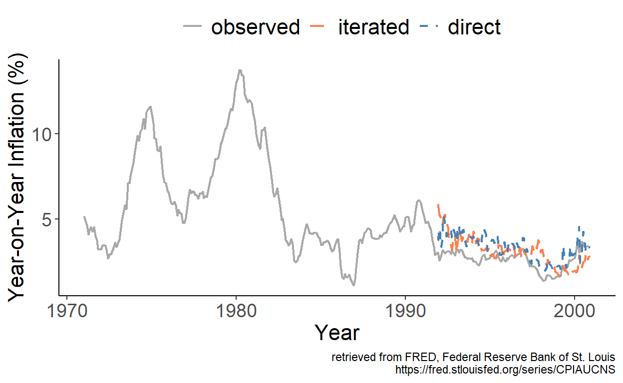
Figure 5.1: Iterated and Direct Forecasts
The foregoing figure illustrates the forecasts, obtained from iterated and direct multi-step forecasting methods. We examine the relative out-of-sample forecast accuracy of the two methods by regressing the loss differential \(d_t=e_{t,d}^2-e_{t,i}^2\) on a constant, where \(t=R+h,\ldots,T\), and where the subscripts \(d\) and \(i\) indicate the direct and iterated multi-step forecasting method, respectively. In this example, as it turns out, we are unable to reject the null hypothesis of equal forecast accuracy as the DM test statistic happens to be -1.18.