Chapter 4 – Generating and Evaluating Forecasts
4.1 Pseudo-Forecasting Routine
Forecast accuracy should only be determined by considering how well a model performs on data not used in estimation. But to assess forecast accuracy we need access to the data, typically from future time periods, that was not used in estimation. This leads to the so-called ‘pseudo forecasting’ routine. This routine involves splitting the available data into two segments referred to as ‘in-sample’ and ‘out-of-sample’. The in-sample segment of a series is also known as the ‘estimation set’ or the ‘training set’. The out-of-sample segment of a series is also known as the ‘hold-out set’ or the ‘test set’.
Thus, we make the so-called ‘genuine’ forecasts using only the information from the estimation set, and assess the accuracy of these forecasts in an out-of-sample setting.
Because forecasting is often performed in a time series context, the estimation set typically predates the hold-out set. In non-dynamic settings such chronological ordering may not be necessary, however.
There are different forecasting schemes for updating the information set in the pseudo-forecasting routine. These are: recursive, rolling, and fixed.
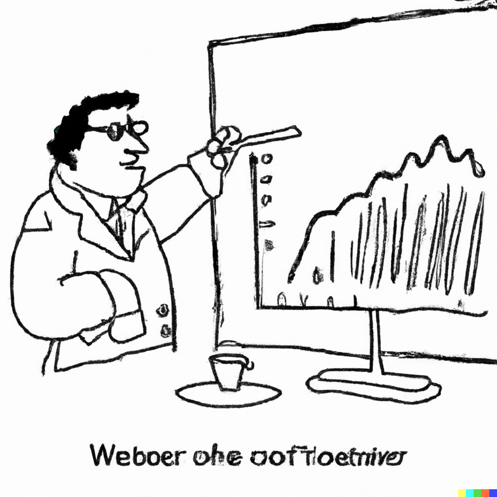
The recursive forecasting environment uses a sequence of expanding windows to update model estimates and the information set.
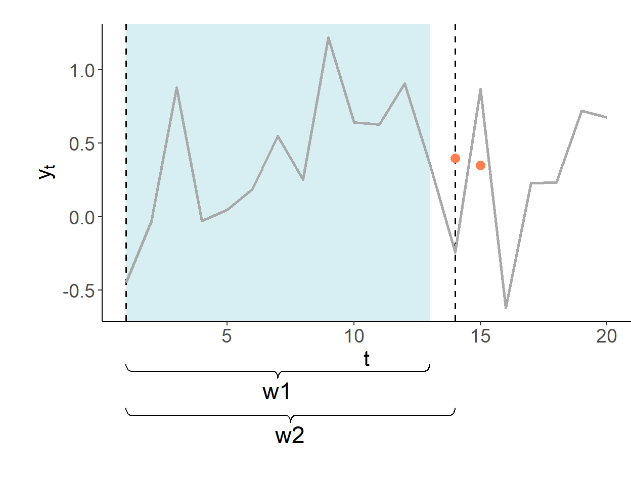
The rolling forecasting environment uses a sequence of rolling windows of the same size to update model estimates and the information set.
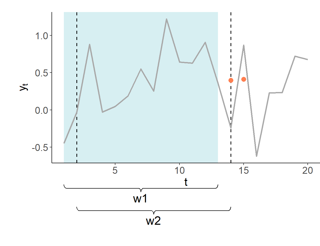
The fixed forecasting environment uses one fixed window for model estimates, and only updates the information set.
The forecasts are made in period 13 for periods 14 and onward. The first estimation window of the pseudo-forecasting routine covers periods one–through–ten. In this illustration, shaded segments illustrate the range of the data used for estimation of model parameters.
4.2 Forecast Assessment
To assess the accuracy of a forecast method, we compare forecast errors from two (or more) methods to each other. Consider a time series, \(\{y_t\}\), with a total of \(T\) observations. To generate genuine forecasts, we decide on the size of the in-sample set consisting of \(R\) observations so that \(R < T\) (typically, \(R \approx 0.75T\)), and the out-of-sample set consisting of \(P\) observations, where \(P=T-R-h+1\) and where \(h\) is the forecast horizon.
For example, if we are interested in one-step-ahead forecast assessment, this way we will produce a sequence of forecasts: \(\{y_{R+1|R},y_{R+2|{R+1}},\ldots,y_{T|{T-1}}\}\) for \(\{Y_{R+1},Y_{R+2},\ldots,Y_{T}\}\).
Forecast errors, \(e_{R+j} = y_{R+j} - y_{R+j|{R+j-1}}\), then can be computed for \(j = 1,\ldots,T-R\).
Two most commonly applied measures of forecast accuracy are the mean absolute forecast error (MAFE) and the root mean squared forecast error (RMSFE): \[\begin{aligned} \text{MAFE} = & \frac{1}{P}\sum_{i=1}^{P}|e_i|\\ \text{RMSFE} = & \sqrt{\frac{1}{P}\sum_{i=1}^{P}e_i^2} \end{aligned}\] The lower is the measure of accuracy associated with a given method, the better this method performs in generating accurate forecasts. As noted earlier, ‘better’ does not mean ‘without errors’.
Forecast errors of a ‘good’ forecasting method will have the following properties:
- zero mean; otherwise, the forecasts are biased.
- no correlation with the forecasts; otherwise, there is information left that should be used in computing forecasts.
- no serial correlation among one-step-ahead forecast errors. Note that \(k\)-step-ahead forecasts, for \(k>1\), can be, and usually are, serially correlated.
Any forecasting method that does not satisfy these properties has a potential to be improved.
The aforementioned three desired properties of forecast errors are, in effect, hypotheses that can be tested. This can be done in a basic regression setting.
4.2.1 Unbiasedness
Testing \(E(e_{t+h|t})=0\). Set up a regression: \[e_{t+h|t} = \alpha+\upsilon_{t+h},\;~~t = R,\ldots,T-h,\] where \(R\) is the estimation window size, \(T\) is the sample size, and \(h\) is the forecast horizon length. The null of zero-mean forecast error is equivalent of testing \(H_0: \alpha = 0\) in the OLS setting. For \(h\)-step-ahead forecast errors, when \(h>1\), autocorrelation consistent standard errors should be used.
4.2.2 Efficiency
Testing \(Cov(e_{t+h|t},\hat{y}_{t+h|t})=0\). Set up a regression: \[e_{t+h|t} = \alpha + \beta \hat{y}_{t+h|t} + \upsilon_{t+h},\;~~t = R,\ldots,T-h.\] The null of forecast error independence of the information set is equivalent of testing \(H_0: \beta = 0\) in the OLS setting. For \(h\)-step-ahead forecast errors, when \(h>1\), autocorrelation consistent standard errors should be used.