Tutorial 7: Vector Autoregression
In this tutorial, we will generate bivariate autocorrelated series, we will apply a system-wide information criterion to select a suitable vector autoregressive model, we will perform an in-sample test of Granger causality, we will obtain and compare one-step-ahead forecasts from competing models using a rolling window procedure, and in so doing we will investigate evidence of out-of-sample Granger causality. To run the code, the data.table, ggplot2 and MASS packages need to be installed and loaded.
Let’s generate a two-dimensional vector of time series that follow a VAR(1) process of the following form: \[\begin{aligned} x_{1t} &= 0.3 + 0.7x_{1t-1} + 0.1x_{2t-1} + \varepsilon_{1t} \\ x_{2t} &= -0.2 + 0.9x_{1t-1} + \varepsilon_{2t} \end{aligned}\] where \(\mathbf{e}_{t} \sim N(\mathbf{0},\Sigma)\), and where \(\Sigma\) is the covariance matrix of the residuals such that \(Cov(\varepsilon_{1,t},\varepsilon_{2,t}) = 0.3\) for all \(t=1,\ldots,180\). (Note: in the code, \(x_1\) is denoted by \(y\) and \(x_2\) is denoted by \(x\)).
n <- 180

R <- matrix(c(1,0.3,0.3,1),nrow=2,ncol=2)
set.seed(1)
r <- mvrnorm(n,mu=c(0,0),Sigma=R)

r1 <- r[,1]
r2 <- r[,2]

x1 <- rep(NA,n)
x2 <- rep(NA,n)

x1[1] <- r1[1]
x2[1] <- r2[1]

for(i in 2:n){
  x1[i] <-  0.3+0.7*x1[i-1]+0.1*x2[i-1]+r1[i]
  x2[i] <- -0.2+0.9*x2[i-1]+r2[i]
}
Generate a vector of some arbitrary dates (e.g., suppose we deal with the monthly series beginning from January 2006), and store these along with \(y\) in a data.table, call it ‘dt’.
Plot the realized time series using a ggplot function. Before plotting, first ‘melt’ the dataset into the ‘long’ format.
dl <- melt(dt,id.vars="date",variable.name="series",value.name="values")

ggplot(dl,aes(x=date,y=values,color=series,linetype=series))+
  geom_line(size=1)+
  scale_color_manual(values=c("powderblue","coral"))+
  labs(x="Year",y="Series")+
  theme_classic()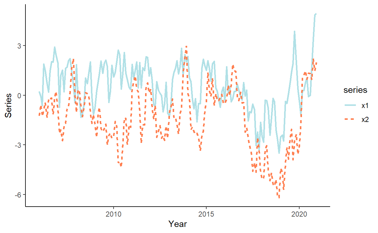
Estimate VAR(1) and VAR(2) by running regressions on each equation separately. Collect residuals and obtain system-wide AIC for each of the two models.
dt[,`:=`(x11=shift(x1,1),x12=shift(x1,2),x21=shift(x2,1),x22=shift(x2,2))]

# VAR(1)
p <- 1
k <- 2

var1.x1 <- lm(x1~x11+x21,data=dt)
var1.x2 <- lm(x2~x11+x21,data=dt)

res1 <- cbind(var1.x1$residuals,var1.x2$residuals)
cov1 <- crossprod(res1)/(nrow(dt)-(p*k^2+k))

AIC1 <- log(det(cov1))+2*(p*k^2+k)/nrow(dt)

# VAR(2)
p <- 2
k <- 2

var2.x1 <- lm(x1~x11+x21+x12+x22,data=dt)
var2.x2 <- lm(x2~x11+x21+x12+x22,data=dt)

res2 <- cbind(var2.x1$residuals,var2.x2$residuals)
cov2 <- crossprod(res2)/(nrow(dt)-(p*k^2+k))

AIC2 <- log(det(cov2))+2*(p*k^2+k)/nrow(dt)

AIC1
## [1] -0.1270596## [1] -0.047212Perform tests of (in-sample) Granger causality in each of the two models. Note, in the case of VAR(1), t tests and F tests are equivalently applicable. In the case of VAR(p), i.e., when \(p>1\), the only appropriate test is an F test for joint significance of the parameters associated with the lags of the potentially causal (in Garanger sense) variable.
##
## Call:
## lm(formula = x1 ~ x11 + x21, data = dt)
##
## Residuals:
##      Min       1Q   Median       3Q      Max
## -2.32279 -0.63680 -0.00953  0.68826  2.63468
##
## Coefficients:
##             Estimate Std. Error t value Pr(>|t|)
## (Intercept)  0.34926    0.11146   3.134  0.00202 **
## x11          0.68903    0.05877  11.725  < 2e-16 ***
## x21          0.11304    0.04509   2.507  0.01308 *
## ---
## Signif. codes:  0 '***' 0.001 '**' 0.01 '*' 0.05 '.' 0.1 ' ' 1
##
## Residual standard error: 0.976 on 176 degrees of freedom
##   (1 observation deleted due to missingness)
## Multiple R-squared:  0.5689, Adjusted R-squared:  0.564
## F-statistic: 116.1 on 2 and 176 DF, p-value: < 2.2e-16##
## Call:
## lm(formula = x2 ~ x11 + x21, data = dt)
##
## Residuals:
## Min 1Q Median 3Q Max
## -2.38491 -0.68087 0.03216 0.66109 2.74762
##
## Coefficients:
## Estimate Std. Error t value Pr(>|t|)
## (Intercept) -0.22353 0.10805 -2.069 0.040 *
## x11 0.05814 0.05697 1.021 0.309
## x21 0.85285 0.04371 19.511 <2e-16 ***
## ---
## Signif. codes: 0 '***' 0.001 '**' 0.01 '*' 0.05 '.' 0.1 ' ' 1
##
## Residual standard error: 0.9461 on 176 degrees of freedom
## (1 observation deleted due to missingness)
## Multiple R-squared: 0.7536, Adjusted R-squared: 0.7508
## F-statistic: 269.2 on 2 and 176 DF, p-value: < 2.2e-16## Analysis of Variance Table
##
## Model 1: x1 ~ x11 + x21
## Model 2: x1 ~ x11
## Res.Df RSS Df Sum of Sq F Pr(>F)
## 1 176 167.64
## 2 177 173.62 -1 -5.9866 6.2852 0.01308 *
## ---
## Signif. codes: 0 '***' 0.001 '**' 0.01 '*' 0.05 '.' 0.1 ' ' 1## Analysis of Variance Table
##
## Model 1: x2 ~ x11 + x21
## Model 2: x2 ~ x21
## Res.Df RSS Df Sum of Sq F Pr(>F)
## 1 176 157.54
## 2 177 158.47 -1 -0.93231 1.0416 0.3089##
## Call:
## lm(formula = x1 ~ x11 + x21, data = dt)
##
## Residuals:
## Min 1Q Median 3Q Max
## -2.32279 -0.63680 -0.00953 0.68826 2.63468
##
## Coefficients:
## Estimate Std. Error t value Pr(>|t|)
## (Intercept) 0.34926 0.11146 3.134 0.00202 **
## x11 0.68903 0.05877 11.725 < 2e-16 ***
## x21 0.11304 0.04509 2.507 0.01308 *
## ---
## Signif. codes: 0 '***' 0.001 '**' 0.01 '*' 0.05 '.' 0.1 ' ' 1
##
## Residual standard error: 0.976 on 176 degrees of freedom
## (1 observation deleted due to missingness)
## Multiple R-squared: 0.5689, Adjusted R-squared: 0.564
## F-statistic: 116.1 on 2 and 176 DF, p-value: < 2.2e-16##
## Call:
## lm(formula = x2 ~ x11 + x21, data = dt)
##
## Residuals:
## Min 1Q Median 3Q Max
## -2.38491 -0.68087 0.03216 0.66109 2.74762
##
## Coefficients:
## Estimate Std. Error t value Pr(>|t|)
## (Intercept) -0.22353 0.10805 -2.069 0.040 *
## x11 0.05814 0.05697 1.021 0.309
## x21 0.85285 0.04371 19.511 <2e-16 ***
## ---
## Signif. codes: 0 '***' 0.001 '**' 0.01 '*' 0.05 '.' 0.1 ' ' 1
##
## Residual standard error: 0.9461 on 176 degrees of freedom
## (1 observation deleted due to missingness)
## Multiple R-squared: 0.7536, Adjusted R-squared: 0.7508
## F-statistic: 269.2 on 2 and 176 DF, p-value: < 2.2e-16## Analysis of Variance Table
##
## Model 1: x1 ~ x11 + x21 + x12 + x22
## Model 2: x1 ~ x11 + x12
## Res.Df RSS Df Sum of Sq F Pr(>F)
## 1 173 166.68
## 2 175 172.78 -2 -6.0971 3.1641 0.04471 *
## ---
## Signif. codes: 0 '***' 0.001 '**' 0.01 '*' 0.05 '.' 0.1 ' ' 1## Analysis of Variance Table
##
## Model 1: x2 ~ x11 + x21 + x12 + x22
## Model 2: x2 ~ x21 + x22
## Res.Df RSS Df Sum of Sq F Pr(>F)
## 1 173 156.76
## 2 175 158.03 -2 -1.2729 0.7024 0.4968Generate a sequence of one-step-ahead forecasts from VAR(1) using the rolling window scheme, where the first rolling window ranges from period 1 to period 120.
R <- 120
P <- nrow(dt)-R

dt$f.a11 <- NA
dt$f.a12 <- NA
dt$f.v11 <- NA
dt$f.v12 <- NA

for(i in 1:P){

  ar1.x1 <- lm(x1~x11,data=dt[i:(R-1+i)])
  ar1.x2 <- lm(x2~x21,data=dt[i:(R-1+i)])

  var1.x1 <- lm(x1~x11+x21,data=dt[i:(R-1+i)])
  var1.x2 <- lm(x2~x11+x21,data=dt[i:(R-1+i)])

  dt$f.a11[R+i] <- ar1.x1$coefficients["(Intercept)"]+ar1.x1$coefficients["x11"]*dt$x1[R-1+i]
  dt$f.a12[R+i] <- ar1.x2$coefficients["(Intercept)"]+ar1.x2$coefficients["x21"]*dt$x2[R-1+i]

  dt$f.v11[R+i] <- var1.x1$coefficients["(Intercept)"]+var1.x1$coefficients["x11"]*dt$x1[R-1+i]+var1.x1$coefficients["x21"]*dt$x2[R-1+i]
  dt$f.v12[R+i] <- var1.x2$coefficients["(Intercept)"]+var1.x2$coefficients["x11"]*dt$x1[R-1+i]+var1.x2$coefficients["x21"]*dt$x2[R-1+i]

}
Calculate the RMSFE measures for restricted and unrestricted models, and compare those to each other to make a suggestion about out-of-sample Granger causality.
dt[,`:=`(e.a11=x1-f.a11,e.a12=x2-f.a12,e.v11=x1-f.v11,e.v12=x2-f.v12)]

# calculate RMSFEs for restricted and unrestricted models
rmsfe_x1.r <- sqrt(mean(dt$e.a11^2,na.rm=T))
rmsfe_x1.u <- sqrt(mean(dt$e.v11^2,na.rm=T))

rmsfe_x2.r <- sqrt(mean(dt$e.a12^2,na.rm=T))
rmsfe_x2.u <- sqrt(mean(dt$e.v12^2,na.rm=T))

rmsfe_x1.r
## [1] 1.134867## [1] 1.104268## [1] 1.00908## [1] 1.011653