Tutorial 10: Combining Forecasts
In this tutorial, we will generate a time series, we will obtain one-step-ahead forecasts from a set of models using a rolling window procedure, we will combine these forecasts and assess the accuracy of the combined forecast. To run the code, the data.table, ggplot2, lmtest, and sandwich packages need to be installed and loaded.
Let’s generate a time series that follow an AR(2) process with the linear trend component as follows: \[y_t = 0.02t-0.0001t^2+1.2y_{t-1}-0.5y_{t-2}+\varepsilon_t\] where \(e_{t} \sim N(0,\sigma^2)\).
n <- 180

set.seed(8)
e <- rnorm(n,0,1)

y <- rep(NA,n)
y[1] <- 0.02*1-0.0001*(1)^2+e[1]
y[2] <- 0.02*2-0.0001*(2)^2+1.2*y[1]+e[2]
for(i in 3:n){
  y[i] <- 0.02*i-0.0001*(i)^2+1.2*y[i-1]-0.5*y[i-2]+e[i]
}
Generate a vector of some arbitrary dates (e.g., suppose we deal with the monthly series beginning from January 2000), store these along with \(y\) in a data.table, call it ‘dt’, and plot the realized time series using ggplot function.
date <- seq(as.Date("2000-01-01"),by="month",along.with=y)

dt <- data.table(date,y)

ggplot(dt,aes(x=date,y=y))+
  geom_line(size=1)+
  labs(x="Year",y="Series")+
  theme_classic()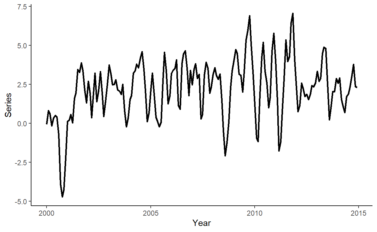
Suppose the candidate models are AR(1), AR(2), and AR(1) with linear trend, and that we want to compare forecasts obtained from these models to those from a random walk process. Generate a sequence of one-step-ahead forecasts using the rolling window scheme, where the size of the rolling window is approximately 75% of the length of the series.
dt[,`:=`(y1=shift(y,1),y2=shift(y,2),y3=shift(y,3),trend=c(1:nrow(dt)))]

R <- round(.75*nrow(dt))
P <- nrow(dt)-R

dt[,`:=`(rw=as.numeric(NA),a1=as.numeric(NA),a2=as.numeric(NA),tr=as.numeric(NA))]

for(i in 1:P){

  dt$rw[R+i] <- dt$y[R+i-1]

  a1 <- lm(y~y1,data=dt[i:(R+i-1)])
  a2 <- lm(y~y1+y2,data=dt[i:(R+i-1)])
  tr <- lm(y~y1+trend,data=dt[i:(R+i-1)])

  dt$a1[R+i] <- a1$coefficients%*%as.numeric(c(1,dt[R+i,c("y1")]))
  dt$a2[R+i] <- a2$coefficients%*%as.numeric(c(1,dt[R+i,c("y1","y2")]))
  dt$tr[R+i] <- tr$coefficients%*%as.numeric(c(1,dt[R+i,c("y1","trend")]))

}
Does either of the considered models ‘statistically significantly’ outperform the random walk?
dt[,`:=`(e_rw=y-rw,e_a1=y-a1,e_a2=y-a2,e_tr=y-tr)]

dt[,`:=`(ld1=e_rw^2-e_a1^2,ld2=e_rw^2-e_a2^2,ldt=e_rw^2-e_tr^2)]

reg_ld1 <- lm(ld1~1,data=dt)
reg_ld2 <- lm(ld2~1,data=dt)
reg_ldt <- lm(ldt~1,data=dt)

lmtest::coeftest(reg_ld1,vcov.=sandwich::vcovHAC(reg_ld1))
##
## t test of coefficients:
##
## Estimate Std. Error t value Pr(>|t|)
## (Intercept) 0.23744 0.16521 1.4372 0.1577##
## t test of coefficients:
##
## Estimate Std. Error t value Pr(>|t|)
## (Intercept) 0.49699 0.27820 1.7865 0.08091 .
## ---
## Signif. codes: 0 '***' 0.001 '**' 0.01 '*' 0.05 '.' 0.1 ' ' 1##
## t test of coefficients:
##
## Estimate Std. Error t value Pr(>|t|)
## (Intercept) 0.27481 0.14690 1.8707 0.06805 .
## ---
## Signif. codes: 0 '***' 0.001 '**' 0.01 '*' 0.05 '.' 0.1 ' ' 1All of the models, on average, generate more accurate forecasts than random walk. None of the models generate statistically significantly (at 5% significance level) more accurate forecast than random walk, based on Diebold-Mariano test applied on quadratic loss function.
Might each model contain some useful information for improving forecast accuracy? Let’s combine the forecasts from the AR(2) and the AR(1) with linear trend using the equal weights scheme and assess the relative accuracy of the combined forecast.
dt$co <- dt$a2*.5+dt$tr*.5
dt$e_co <- dt$y-dt$co

dt$ldc <- dt$e_rw^2-dt$e_co^2

reg_ldc <- lm(ldc~1,data=dt)

lmtest::coeftest(reg_ldc,vcov.=sandwich::vcovHAC(reg_ldc))
##
## t test of coefficients:
##
## Estimate Std. Error t value Pr(>|t|)
## (Intercept) 0.48226 0.22397 2.1532 0.03682 *
## ---
## Signif. codes: 0 '***' 0.001 '**' 0.01 '*' 0.05 '.' 0.1 ' ' 1