Choice and Efficiency
Kolstad (2010, Chapters 2 & 3); Keohane and Olmstead (2016, Chapter 4)
Utility and Indifference of Choices
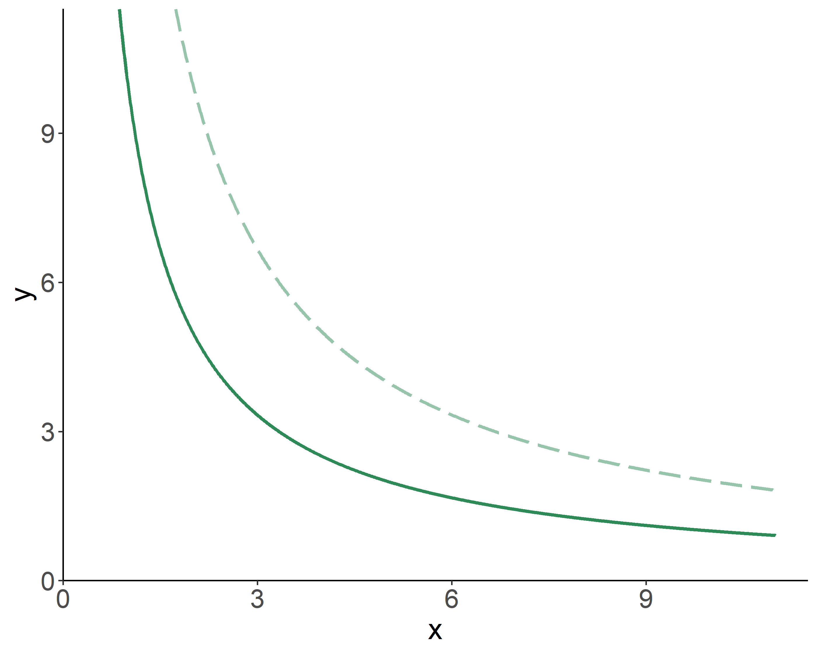
People face choices all the time. These choices typically involve an array of goods, typically the so-called market goods (e.g., cookies, cars), but also environmental goods (e.g., clean water, fresh air). As with market goods, people enjoy—or get (positive) utility from—environmental goods. In what follows, we shall denote a (composite) market good with \(x\), and an environmental good with \(y\).
Intuitively, because environmental pollution is a by-product of production of a market good, a consumer is left with a choice of giving up some of their desired good, to mitigate the damage to the environmental good. Note that different people (e.g., person \(i\) and person \(j\)) may choose to consume different amounts of the market good: \(x_i\neq x_j\); but everyone will consume the same amount of the environmental good: \(y_i=y_j=y\). Even so, the value, or the utility attained from this environmental good will vary among individuals.
There are many sources of utility from environmental goods (or negative utility from environmental bads):
- health benefits (e.g., lower incidence of respiratory problems);
- productivity value (e.g., greenhouse gases increase temperature, which adversely impacts agricultural production);
- use value (e.g., whale watching);
- existence value (feeling good about clean environment);
- altruism (feeling good knowing others enjoy clean environment)
Thus, the benefit provided to a person \(i\) by consuming the market and environmental goods is represented by a utility function: \(u_i(x_i,y)\).
Prices and the Optimal Choice
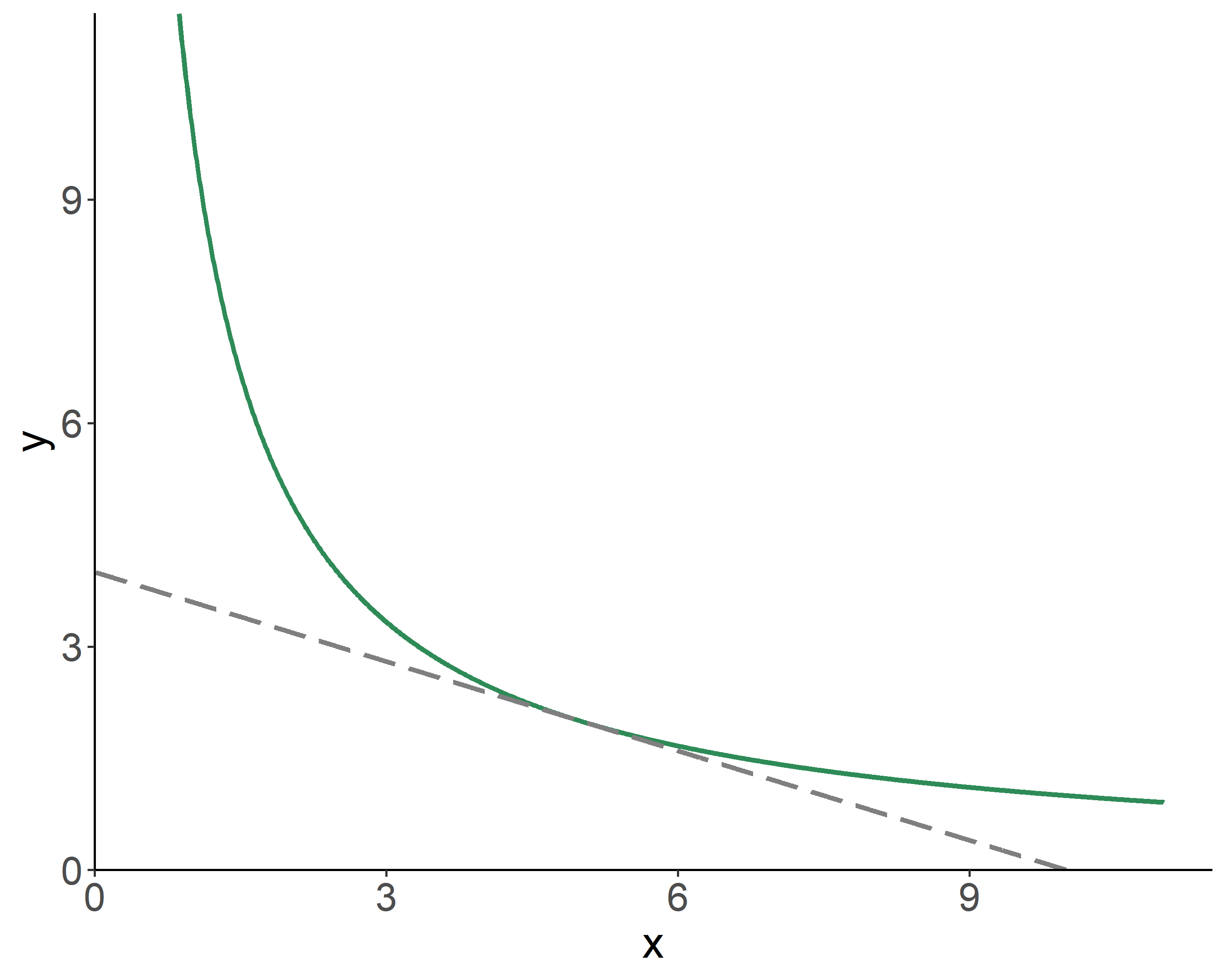
From an array of options, a person will choose an optimal bundle of composite market and environmental goods, \(\left\{x^*,y^*\right\}\), such that their utility is maximized given their income, \(M\), and the prices of these two goods, \(p_x\) and \(p_y\). In other words, an individual’s objective is to maximize the utility subject to the budget constraint.
Mathematically: \[\max_{x,y}U(x,y),\;~~\mbox{s.t.}\;~p_{x}x+p_{y}y=M.\] The optimization leads to: \[\frac{MU_x}{MU_y} = \frac{p_x}{p_y}\] where the ratio of the two marginal utilities is referred to as the marginal rate of substitution, \(MRS_{x,y}\), which indicates the amount of units of \(y\) a consumer is willing to give up to get a unit of \(x\).
Efficiency in Exchange
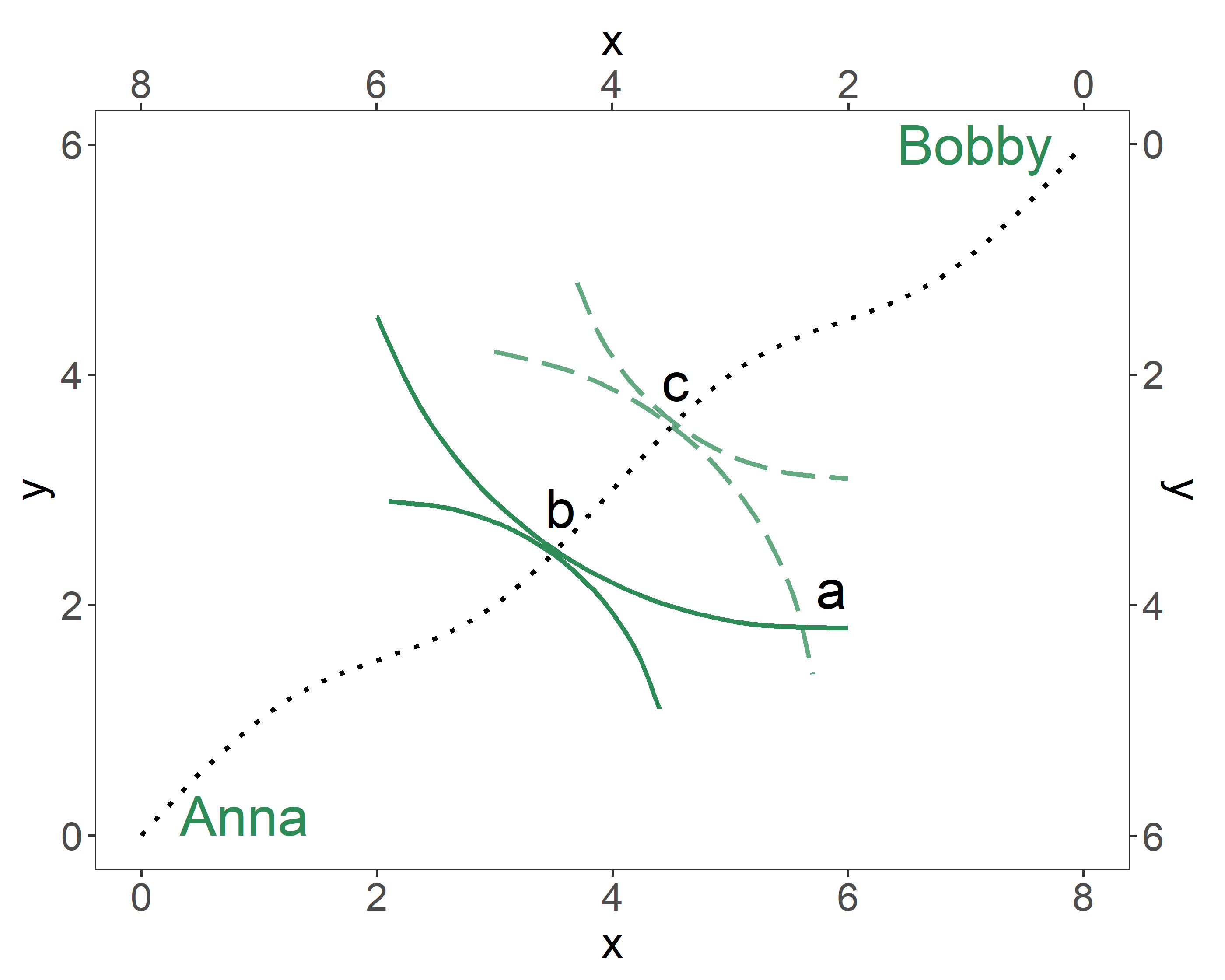
Consider achieving efficiency (in exchange of goods) in a two-person economy. In the illustrated Edgeworth Box, any point on the plane represents an allocation of the two goods between the two individuals. The allocations along the contract curve—the dotted line on the graph—are Pareto optimal. For any given endowment (i.e., initial allocation), efficiency can be achieved along an array of points—the contract curve—where indifference curves of the two individuals are tangent to one another.
Social Choice Mechanisms
The foregoing discussion helps us understand (or, to some extent, conceptualize) an individual’s preferences for a given bundle of market and environmental goods. But how about the society as a whole?
We can examine everyone’s preferences, and if all happen to prefer some alternative over all other alternatives, we may conclude that the society as a whole prefers that alternative. This is also known as the Pareto criterion for social choice.
Allocations on the Pareto frontier are efficient, i.e., Pareto optimal. Pareto optimality implies an allocation of goods at which it is impossible to make anyone better off, without making someone worse off. Pareto frontier is, in essence, the contract curve.
An allocation is inefficient if it is interior to Pareto frontier. In such instance, a Pareto improvement is possible. Pareto improvement implies an action that harms no one, and benefits at least one individual.
In the provided graph, the allocations \(X\), \(Y\), and \(Z\), are inefficient, and only the allocation \(Z\), is efficient. \(Y\), though inefficient, is Pareto improvement over \(X\). In fact, all allocations in the shaded region are Pareto improvements over \(X\).
The Pareto criterion is unanimity rule. For allocations \(a\) and \(b\), everyone must prefer the former to the latter for \(a\) to be Pareto preferred to \(b\). Because of this rule, decisions tend to be biased toward status quo, when Pareto criterion is applied to make societal decisions.
An alternative rule—that circumvents the issues associated with Pareto criterion—is unanimity with side payments; that is, when member of society are allowed to transfer resources to increase the unanimity of opinion on alternative allocations. This approach, inherently, accounts for the extent to which individuals prefer one option to another. The rule leads to a potential Pareto improvement, which implies an action that harms no one, and benefits at least one individual, after a set of net-zero transfers (side payments) have taken place.
Another mechanism—that relaxes the unanimity rule—is a voting mechanism based on the majority rule. For allocations \(a\) and \(b\), if the majority prefers the former to the latter, we conclude that \(a\) is preferred to \(b\), even though there may be people in the society who strongly prefer \(b\) to \(a\).
Social Welfare Functions and Impossibility Theorem
A social welfare function is a way of representing societal preferences, akin to a utility function for individual preferences. If \(U_i(a)\) is the utility that a person \(i\) derives from choice \(a\), then \(a\) is said to be socially preferred to \(b\) if \(W[U_i(a):i=1,\ldots,N] > W[U_i(b):i=1,\ldots,N]\), where \(W[\cdot]\) is a social welfare function that summarizes the distribution of individual utilities in the society. Some of the well–known social welfare functions are:
- Utilitarian: \(W(U_i:i=1,\ldots,N) = \sum_i \theta_i U_i;\;~ \theta_i \ge 0, \sum_i\theta_i=1\)
- Egalitarian: \(W(U_i:i=1,\ldots,N) = \sum_i U_i-\lambda\sum_i[U_i-\min(U_i)]\)
- Rawlsian: \(W(U_i:i=1,\ldots,N) = \min(U_i)\)
For a social choice mechanism to work, it should satisfy the following assumptions:
- Completeness—we should be able to compare alternatives.
- Unanimity—if everyone in the society prefers \(a\) to \(b\), then the society should prefer \(a\) to \(b\).
- Nondictatorship—no one’s preferences should be exactly the same as those of the society.
- Universality—any possible individual rankings of alternatives is allowed.
- Transitivity—if \(a\) is socially preferred to \(b\), and if \(b\) is socially preferred to \(c\), then \(a\) should be socially preferred to \(c\).
- Independence of Irrelevant Alternatives—social preference between two alternates should only depend on people’s preferences for these two, regardless of their preferences for any other alternatives.
These are the axioms put forward by Kenneth Arrow. In what became to be known as Arrow’s Impossibility Theorem he proved that there is no rule satisfying all six assumptions that can convert individual preferences into a social preference ordering.
3.4 Social Choice Mechanisms
The foregoing discussion helps us understand (or, to some extent, conceptualize) an individual’s preferences for a given bundle of market and environmental goods. But how about the society as a whole?
We can examine everyone’s preferences, and if all happen to prefer some alternative over all other alternatives, we may conclude that the society as a whole prefers that alternative. This is also known as the Pareto criterion for social choice.
Allocations on the Pareto frontier are efficient, i.e., Pareto optimal. Pareto optimality implies an allocation of goods at which it is impossible to make anyone better off, without making someone worse off. Pareto frontier is, in essence, the contract curve.
An allocation is inefficient if it is interior to Pareto frontier. In such instance, a Pareto improvement is possible. Pareto improvement implies an action that harms no one, and benefits at least one individual.
Figure 3.4: Pareto Frontier
In the provided graph, the allocations \(X\), \(Y\), and \(Z\), are inefficient, and only the allocation \(Z\), is efficient. \(Y\), though inefficient, is Pareto improvement over \(X\). In fact, all allocations in the shaded region are Pareto improvements over \(X\).
The Pareto criterion is unanimity rule. For allocations \(a\) and \(b\), everyone must prefer the former to the latter for \(a\) to be Pareto preferred to \(b\). Because of this rule, decisions tend to be biased toward status quo, when Pareto criterion is applied to make societal decisions.
An alternative rule—that circumvents the issues associated with Pareto criterion—is unanimity with side payments; that is, when member of society are allowed to transfer resources to increase the unanimity of opinion on alternative allocations. This approach, inherently, accounts for the extent to which individuals prefer one option to another. The rule leads to a potential Pareto improvement, which implies an action that harms no one, and benefits at least one individual, after a set of net-zero transfers (side payments) have taken place.
Another mechanism—that relaxes the unanimity rule—is a voting mechanism based on the majority rule. For allocations \(a\) and \(b\), if the majority prefers the former to the latter, we conclude that \(a\) is preferred to \(b\), even though there may be people in the society who strongly prefer \(b\) to \(a\).