Chapter 7 Regulation with Information Asymmetry
Kolstad (2010, Chapters 12 & 15)
7.1 Imperfect Competition
When markets are not competitive, a host of efficiency problems arise, which, in turn, amplify the issues of environmental regulation. A case in point will be illustrated using two different scenarios: (i) a monopolist in the goods market that is one of many polluters; and (ii) a competitive firm in the goods market that is the only polluter.
7.1.1 Monopolist in Production
Consider a steel manufacturer that also emits pollution. There are many other polluters in the region, but only one steel manufacturer. In absence of regulation, the monopolist will produce where the marginal revenue and the unregulated marginal costs are equal.
The regulation will shift the marginal cost curve upward, and the firm will produce where the marginal revenue and the regulated marginal costs are equal. Turns out, the emission fee has made matters worse.
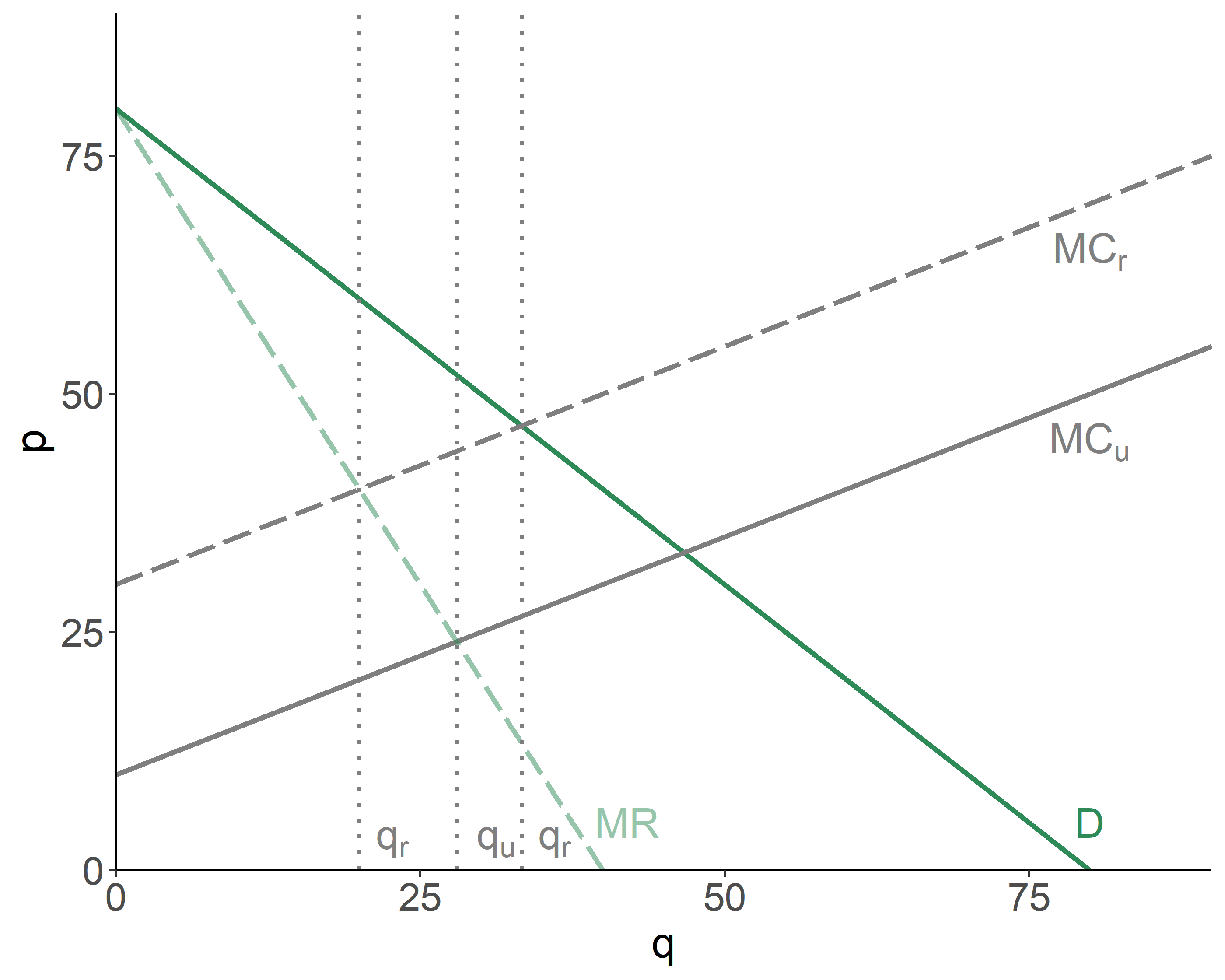
Figure 7.1: Monopolist in Production and Pigovian Tax
The intuition behind this is simple: a monopolist has already lowered output below the competitive levels (which happen to be larger than the socially optimal levels). The imposition of the emission fee further restricts output, and in so doing may just overdo it.
7.1.2 Monopolist in Emission
Consider a firm, which is competitive in the goods market, but is a sole emitter of pollution in the region. That is, the firm is a monopolist in emission. The regulator imposes the emission tax, by setting it equal to the marginal damage of pollution. The firm, being able to observe the slope of the marginal damage function, will end up producing at the level that is below the efficient amount of pollution.
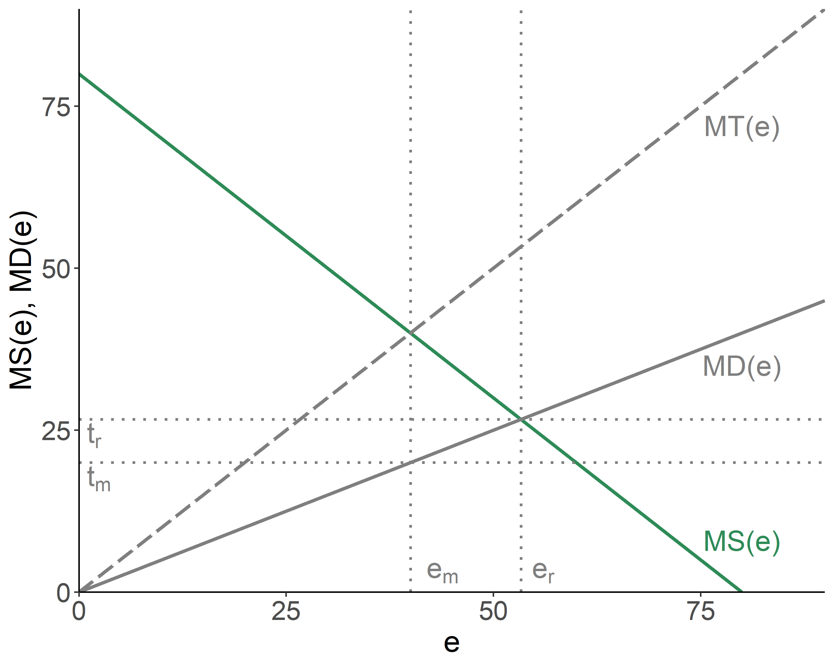
Figure 7.2: Monopolist in Emission and Pigovian Tax
7.2 Limited Information on Pollution Control
Thus far we have assumed that a regulator knows exactly what pollution control costs are. A more realistic scenario, however, is that the regulator only possesses a limited fraction of the polluter’s private information on control costs. In such case, a polluter may benefit from strategically misstating the costs. Questions to be addressed, then, are whether the information uncertainty related to control costs favors the use of emission permits vs. fees as a more adequate means of regulation, and also whether there are benefits to an ex-ante communication (information sharing) between a polluter and a regulator.
Suppose there are two types of polluters: those with high marginal savings from emission, \(MS_H(e)\), and those with low marginal savings from emission, \(MS_L(e)\). A single emission fee, \(\hat{\tau}\), thus will be either too low or too high, depending on the polluter type. Either way, there will be efficiency losses.
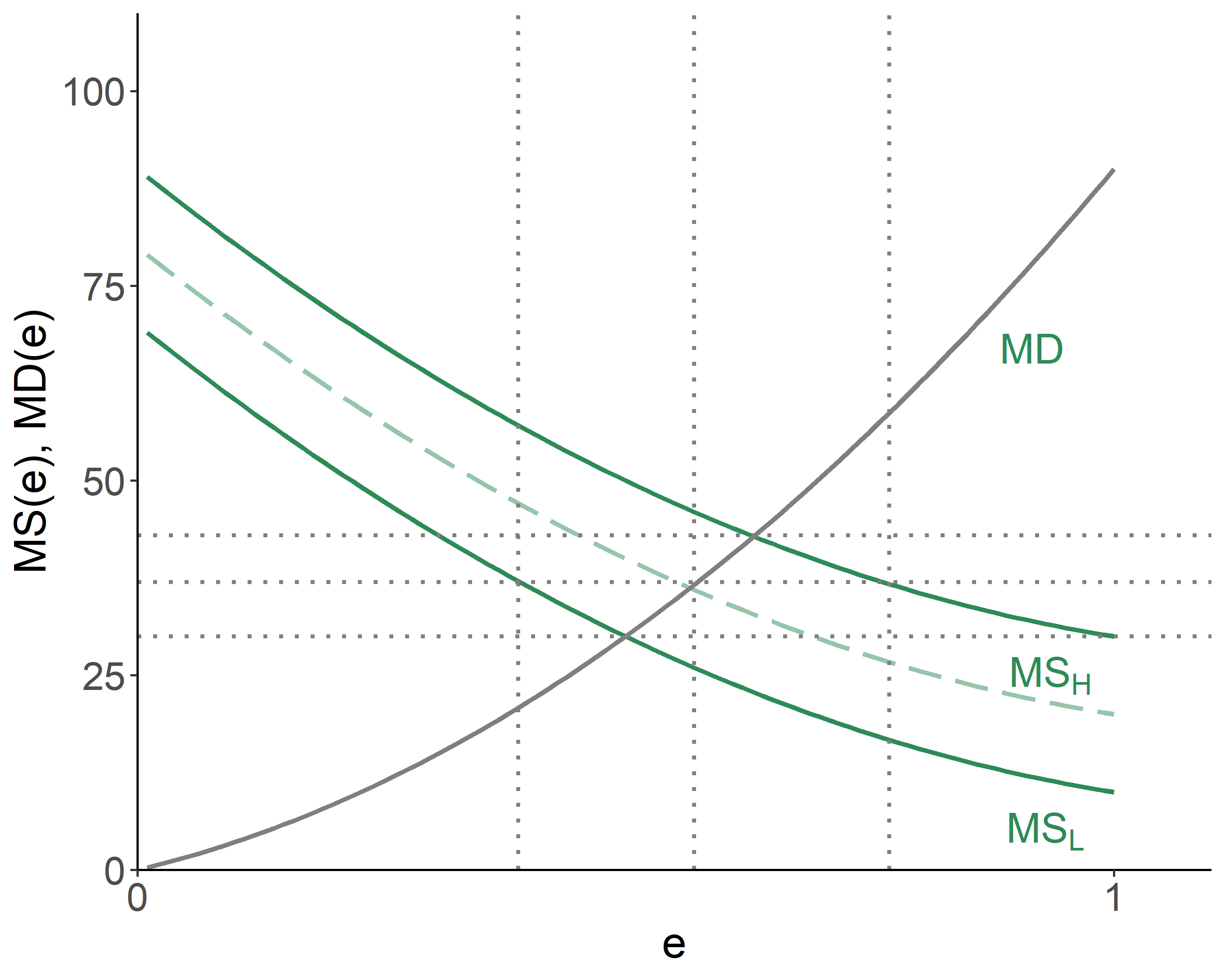
Figure 7.3: Efficiency Losses
If a regulator knew exactly the type of a polluter, it would impose \(\tau_H^*\) on high-cost polluters, and \(\tau_L^*\) on low-cost polluters, and there would have been no efficiency losses. The issue exists, however, because polluters have incentives to misstate their actual type:
- if a regulator were to impose emission fees, a rational polluter would claim they are low-cost, regardless of their actual type;
- if a regulator were to introduce permits, a rational polluter would claim they are high-cost, regardless of their actual type.
One way to ‘correct’ the aforementioned adverse selection issue is by introducing a reward system of some sort for telling the truth. Consider the case of quantity regulations. Suppose a regulator is willing to introduce a reward, \(R\), to motivate truth-telling. So, polluters who claim they are high-cost get paid \(R_H\), and polluters who claim they are low-cost get paid \(R_L\). In fact, we can set \(R_H=0\) (recall: polluters have an in incentive to claim they are high-cost).
Each type of firm will tell the truth as long as that is the optimal strategy after the award has been factored in. For a high-cost firm, this means: \[C_H(e_H) < C_H(e_L)-R_L,\] and for a low-cost firm, this means: \[C_L(e_L)-R_L < C_L(e_H).\] Putting the two together, we obtain: \[C_L(e_L) - C_L(e_H) < R_L < C_H(e_L) - C_H(e_H)\]
Rewards aside, the benefit of lying for a low-cost firm is given by the area under their marginal savings curve, \(MS_L(e)\), and between the low and high levels of emission (respectively denoted by \(e_L\) and \(e_H\)); the benefit of telling the truth for a high-cost firm is given by the area under their marginal savings curve, \(MS_H(e)\), and between the low and high levels of emission.
7.3 Permits vs. Fees
In absence of information asymmetry we saw that a regulator can reach the same outcome, in terms of emission levels, either with emission fees or emission permits. Uncertainty over emission costs, however, may distort such equivalence.
Consider a regulator and a firm. The regulator is aware that the firm can be of the high-cost or the low-cost marginal savings type. But unknown to the regulator remains the exact type of the firm. The regulator can implement either of the two options of emission control—a fee or a permit. But which one of these two is preferred? Martin Weitzman addressed this question in 1974, which led to what is now known as the Weitzman’s Theorem: with uncertainty over emission control costs, emission permits are preferred when marginal damages are more steeply sloped than marginal savings associated with emissions; otherwise, emission fees are preferred.
The issue with emission fees or permits is that neither of the two types of regulations has a flexibility to enforce pollution control, when it is relatively cheap to do so, but be a little more lenient, otherwise. It is, however, possible to introduce a hybrid regulation, where the permit system is coupled with the fee/subsidy mechanism.
The regulatory scheme is such that the firm is told to emit \(e^*\). If it emits less, it will receive subsidy, \(\sigma\), for each unit of pollution under the limit, and if it emits more, it will pay fee, \(\tau\), for each unit of pollution over the limit.
With such mechanism in place, if the firm’s actual marginal savings are low, they will choose to emit \(\hat{e}_L\) and collect subsidy. If, on the other hand, the firm’s marginal savings are high, they will emit \(\hat{e}_H\), which is above the allowed limit, and just pay the penalty for the difference.
The hybrid regulation allows us to achieve complete efficiency when there are only two marginal savings schedules.
When there are more than two types of firms—which is a more likely scenario—the hybrid regulation will not facilitate complete efficiency, but it will still do better than a pure emission fee or a pure emission permit scheme.
References
Kolstad, Charles D. 2010. Environmental Economics. 2nd ed. Oxford University Press.