Chapter 8 Regulation Across Space

Kolstad (2010, Chapter 14)

One of the crucial dimensions of pollution manifestation is space—the degree of exposure to pollution often highly depends on location of those exposed. This complicates the regulator’s task to optimally control pollution emission.

8.1 Emission and Ambient Concentration

Suppose there are several sources of emission, \(e_i\), where \(i=1,\ldots,n\). Each of them, to some extent, impact the air quality at some site, \(v_s\). We can express this relationship as follows: \[v_s = \sum_{i=1}^{n}a_{is}e_i,\] where \(a_{is}\) is the transfer coefficient that links the emission from a source \(i\) with the ambient concentration at a receptor’s site \(s\). For example, \(a_{is}\) can be a function of distance between \(e_i\) and \(v_s\). The concept of the transfer coefficient is particularly useful when the linearity assumption is maintained in the relationship between emissions and pollution.

Recall, the efficient amount of pollution involves equating marginal damages with marginal savings of emission. But, the marginal damage is, actually, measured in terms of ambient pollution. The relationship between the marginal damage in terms of emission from source \(i\), and the marginal damage in terms of ambient concentration at a receptor’s site (to keep things simple we shall assume a single receptor, and drop subscript \(s\) from here forward), can be given by: \[MD(e_i) = a_{i}MD(v),\;~~i=1,\ldots,n.\]

Recognize that for any source, \(i\), \(MS(e_i) = MD(e_i)\); substitute it into the above equation and divide through by \(a_{i}\) to obtain: \[MS(e_i)/a_{i} = MD(v),\;~~i=1,\ldots,n.\] As it follows, two conditions are necessary for efficiency: (i) normalized marginal savings must be equalized for all sources; and (ii) normalized marginal savings must be equal to the marginal damage.

8.2 Ambient–Differentiated Emission Fees

When emission fees are imposed, the firms will respond by minimizing their total costs associated with emission, resulting in: \[MS(e_i) = t_i,\;~\forall\;i.\] It then follow that: \[t_i = a_i MD(v)\] and, to hold the equimarginal principle, \[t_i/a_i = t_j/a_j,\;~~\forall\;i,j.\] That is, the emission fees levied on the firms must be equal, after normalizing by the transfer coefficients.

While the ambient-differentiated emission fees can achieve efficiency, sometimes it is too complicated to vary the emission fee across locations, perhaps due to uncertainty about the transfer coefficients, or perceived unfairness to differentiate fees across firms.

Consider a two-firm scenario, and suppose they have the same marginal savings, but the transfer coefficients vary, resulting in different marginal damage curves. If a regulator were to differentiate, it would set fees at \(t_1\) and \(t_2\), respectively yielding emissions of \(e_1\) and \(e_2\), and incurring no losses in efficiency.

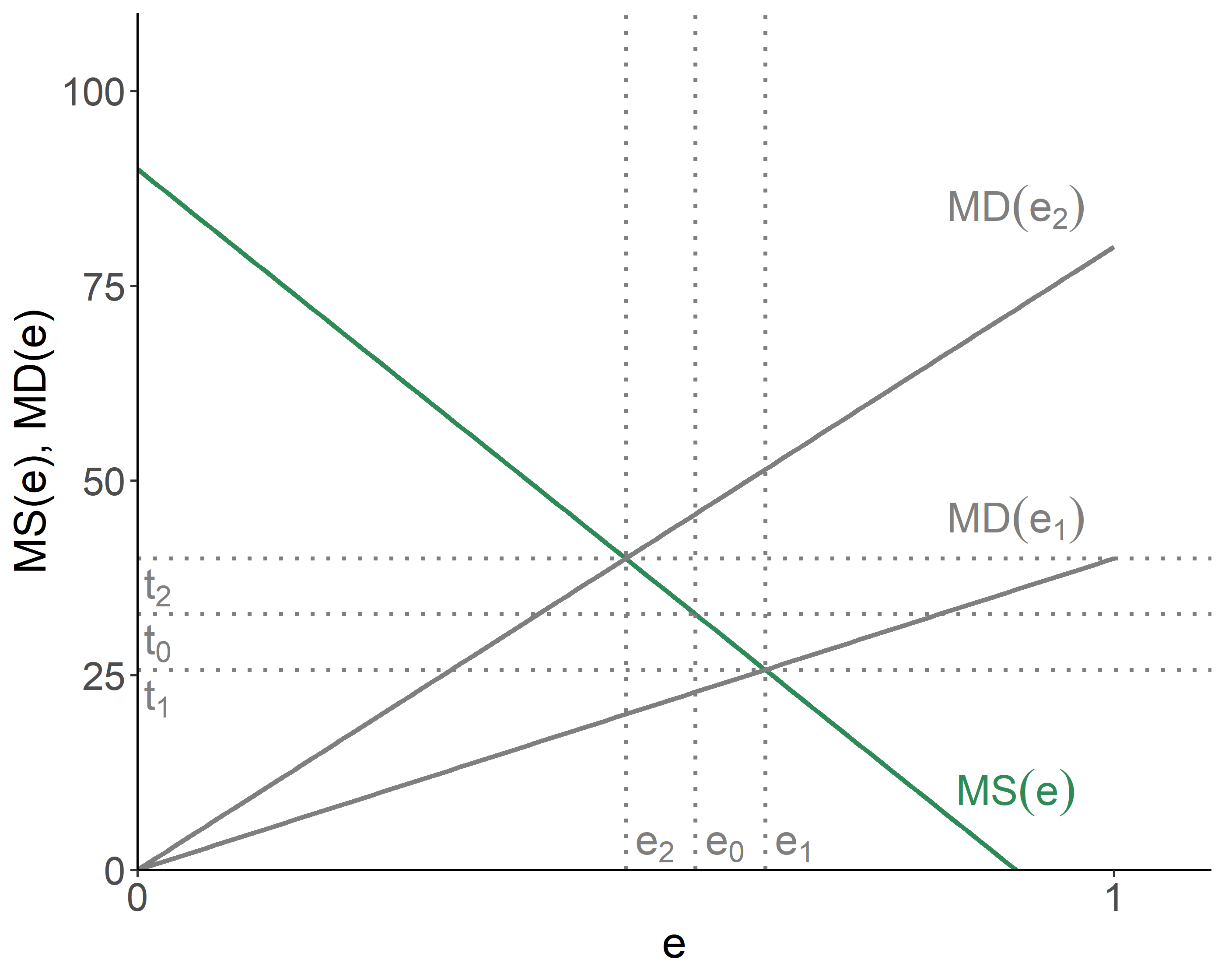
Figure 8.1: Inefficiency of the Uniform Tax

But if a regulator were to use a uniform tax, \(t_0\), both firms would emit the same amount of pollution, \(e_0\), which will result in efficiency losses depicted by: (1) the area between \(e_0\) and \(e_1\), below \(MS(e)\) and above \(MD(e_1)\); and (2) the area between \(e_0\) and \(e_2\), above \(MS(e)\) and below \(MD(e_2)\). If such uniform fee were to be the regulator’s only option, the ‘optimal’ tax would be the one that minimizes the said efficiency losses.

8.3 Marketable Ambient Permits

An emission permit system—that take into account the effect of ambient concentration in the affected locations—is somewhat more complicated, but (in theory) can work just as well as ambient-differentiated emission fees.

Consider a case of two firms and one receptor. If a regulator (randomly) assigns a total of \(L=L_1+L_2\) permits to these firms, the questions to be answered will be: (i) what will the price of permits be? and (ii) how much will each firm emit?

Let \(r\) denote the price of permits, and \(l_1\) and \(l_2\) denote the number of permits eventually held by the firms. Note that: \(l_1=a_1 e_1\) and \(l_2=a_2 e_2\), resulting in \(a_1 e_1 + a_2 e_2 =L\). A firm’s total costs are: \[TC(e_i) = C(e_i)+(a_i e_i - L_i)r,\;~~i=1,2.\] Cost minimization (with respect to \(e_i\)) results in the optimality conditions: \[MS(e_i)/a_i = r,\;~~i=1,2.\] We thus can solve the three equations for three unknowns (\(e_1\), \(e_2\), and \(r\)).

8.4 Zonal Instruments

There can be a middle ground between completely undifferentiated emission fees or permits (i.e., where space is ignored) and ambient fees or permits.

In the case of fees, a region is divided into zones. Within each zone, the same emission fee applies, but fees may vary across the zones. The advantage of such zonal system is more flexibility, resulting in efficiency gains (over the undifferentiated system). The disadvantages are those inherited from the ambient fee system (note that as zones become small and numerous, a zonal fee system, in essence, becomes an ambient fee system).

As for permits, within a zone, they are traded on a 1-for-1 basis. Across the zones, however, a permit trading system applies different transfer coefficients for different zones. There are efficiency gains from a zonal system, accompanied by disadvantages due to complexity associated with the ambient permit system.

References

Kolstad, Charles D. 2010. Environmental Economics. 2nd ed. Oxford University Press.